ML Classifier Models: Fraud Detection

In this project, a dataset containing credit card transactions is examined with the goal of training and testing a machine learning classifier models: K-Nearest Neighbors (KNN). The objective is to predict which transactions are likely to be fraudulent.

After training the model, we will evaluate its performance using a confusion matrix and accuracy metrics. This assessment will help us determine if the model is a suitable choice for accurately identifying fraudulent transactions.

Step 1: Import Libraries

import pandas as pd
import matplotlib.pyplot as plt
import numpy as np
from sklearn.model_selection import train_test_split
from sklearn.neighbors import KNeighborsClassifier
import seaborn as sns
from sklearn.neighbors import KNeighborsClassifier
from sklearn.model_selection import cross_val_score, KFold

Step 2: EDA
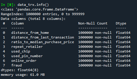
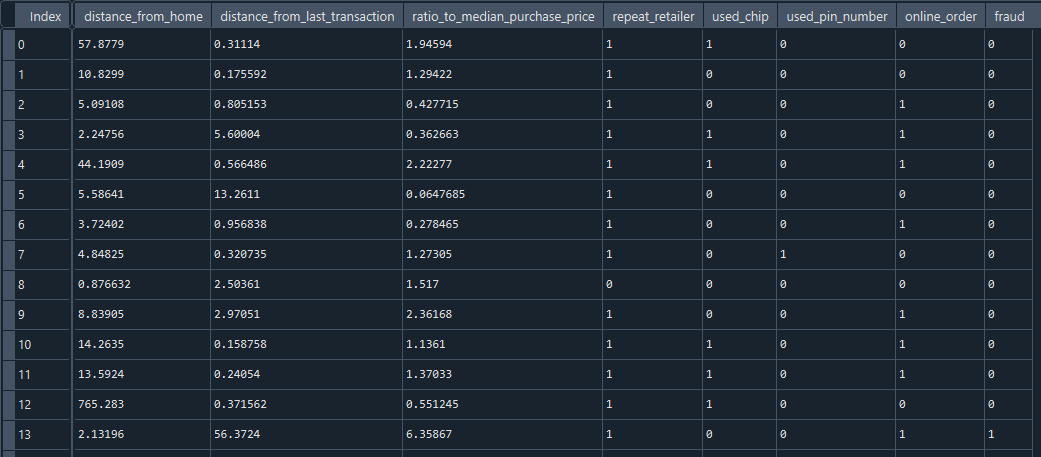
In this step we are reading in the credit card transactions dataset and understanding the structure of the data.

data_trx = pd.read_csv(r"creditcard_trx.csv")
data_trx.shape
data_trx.info()
data_trx.head()

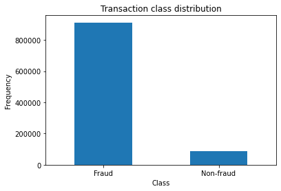
Next lets breakdown the number of fraudulent cases in the dataset. <br>

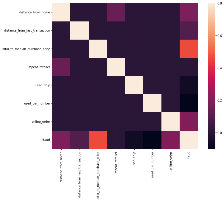
Correlation Heatmap

Next lets plot a correlation heatmap to represent the data in data_trx dataset <br>

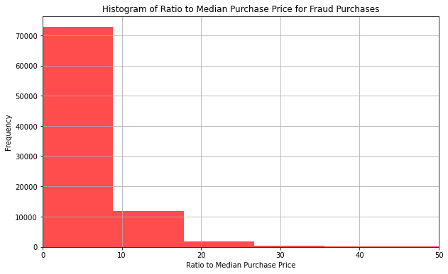
Median fraudulent Purchase Price

Step 3: Pre-processing

Read the features and target values into X and y respectivley

X = data_trx.drop("fraud", axis=1).values
y = data_trx["fraud"].values

This step will split the data into training and test sets

X_train, X_test, y_train, y_test = train_test_split(X, y, test_size=0.2, random_state=42, stratify=y)

Step 4: Building a KNN Classifier Model
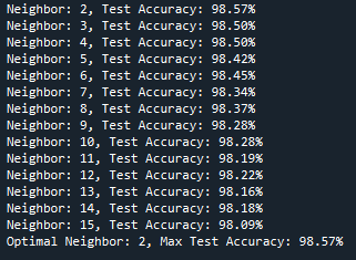
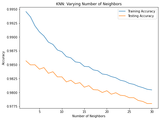
This block of code creates an array of train and test accuracies, sets up a KNN Classifier, and loops through values of k from 2-30.

neighbors = np.arange(2, 31)
train_accuracies = {}
test_accuracies = {}

for neighbor in neighbors:

    knn = KNeighborsClassifier(n_neighbors=neighbor)
    knn.fit(X_train, y_train)

    train_accuracies[neighbor] = knn.score(X_train, y_train)
    test_accuracies[neighbor ]= knn.score(X_test, y_test)

Printing the neighbor value and corresponding test accuracy as a percentage:

Visualizing the test accuracies with various k values

Step 5: Evaluating Classifier Metrics
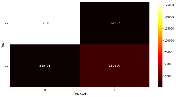
From the analysis we know that the optimal value for k=2. So lets evaluate the models performance metrics using this k value.

knn = KNeighborsClassifier(n_neighbors=2)
#knn = neighbors.KNeighborsClassifier(n_neighbors = 2)
knn.fit(X_train, y_train)
y_pred = knn.predict(X_test)

precision_score(y_test, y_pred)

Importing the confusion matrix library and printing out the matrix

from sklearn.metrics import classification_report, accuracy_score, confusion_matrix, precision_score
cm = confusion_matrix(y_test, y_pred)
cm

In the context of fraud detection or any binary classification problem, the confusion matrix is used to assess how well the model is performing in terms of identifying true cases (fraud) and true non-cases (non-fraud), as well as the errors (false positives and false negatives) it makes. The goal is to minimize false positives and false negatives while maximizing true positives and true negatives.

True Positives (TP): 15,378
This is the number of instances that are actually positive (fraud cases) and are correctly predicted as positive by the model.

True Negatives (TN): 181,761
This is the number of instances that are actually negative (non-fraud) and are correctly predicted as negative by the model.

False Positives (FP): 758
This is the number of instances that are actually negative but are incorrectly predicted as positive by the model. These are also known as Type I errors or “false alarms.”

False Negatives (FN): 2,103
This is the number of instances that are actually positive (fraud) but are incorrectly predicted as negative by the model. These are also known as Type II errors or “missed cases.”

Recommendation
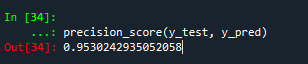
The model’s precision score of 95% and the confusion matrix show that it’s doing an excellent job at accurately identifying positive cases (such as fraud) with very few false positives. This makes it well-suited for applications where precision is critical, like fraud detection.

For more information head over to my Github