
In this project, we will leverage a dataset containing various features like beats per minute (bpm), energy, decibels (dB), acoustic characteristics, and more. The objective is to employ these features to make predictions for the target variable, which is the popularity of songs.
Two regression models, linear regression and ridge regression, will be utilized to train the dataset. The performance of both models will be compared through an evaluation of key metrics like Root Mean Square Error (RMSE) and the coefficient of determination (R^2). Following this analysis, it will be possible to provide a recommendation regarding which model offers superior predictions for song popularity when applied to a test dataset.
Step 1: Import Libraries
import pandas as pd
import matplotlib.pyplot as plt
import numpy as np
from sklearn.model_selection import train_test_split
from sklearn.neighbors import KNeighborsClassifier
import seaborn as sns
from sklearn.neighbors import KNeighborsClassifier
from sklearn.model_selection import cross_val_score, KFold
Step 2: EDA
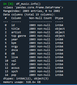
df_music.info()
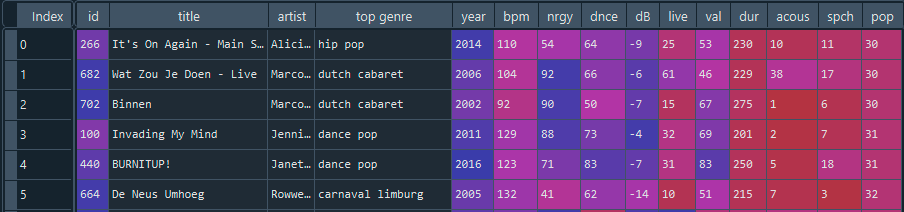
df_music.head()
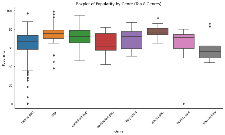
Using seaborn the top 8 genres were plotted against their popularity
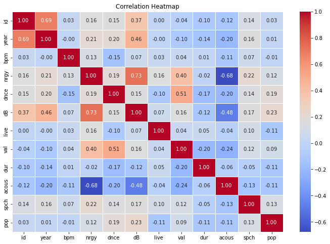
Correlation Heatmap
Next lets plot a correlation heatmap to represent the data in df_music
Scatter Matrix
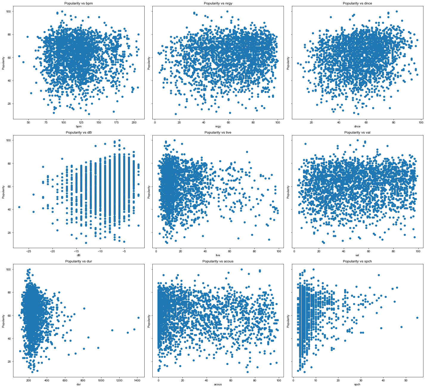
Using a scatter matrix allows us to analyze the relationship between the various features and the target variable in this case song popularity.
From the matrix wee can see the most of the relationships are non-linear.
Step 3: Pre-processing
Delete ID, Title, artist, and year
df_music.drop(columns = ['id', 'title', 'artist', 'year'], inplace = True)
This step will encode dummy variables ie. it will convert the text genre categories into binary 0 or 1 values
music_dummies=pd.get_dummies(df_music['top genre'],drop_first=True)
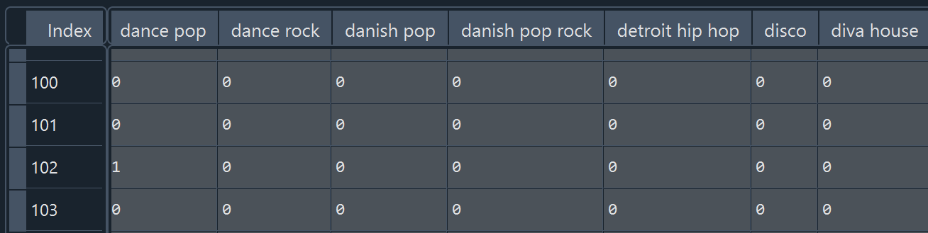
print(music_dummies.head())
Each genre category is now encoded as a 0 or 1. For example in row 102 the genre is ‘dance pop’ therefore this column will contain a 1 with all other genre categories containing a 0.
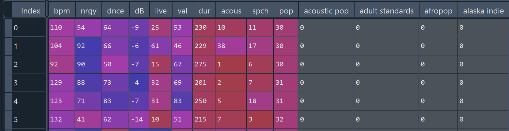
Bring these new columns into the df_music dataframe and display the appended df_music dataframe
df_music=pd.concat([df_music,music_dummies],axis=1)
Step 4: Building a Linear Regression Model
Split the features and target variables into X and y respectively
X = df_music.drop("pop", axis=1).values
y = df_music["pop"].values
Instantiate a linear regression model
reg=LinearRegression()
Perform a 10-fold cross-validation to ensure that data is tested on multiple sets
kf = KFold(n_splits=10, shuffle=True, random_state=5)
Evaluating Linear Regression Metrics
cv_results=cross_val_score(reg, X_train,y_train,cv=kf)
cv_results_MSE=cross_val_score(reg, X_train,y_train,cv=kf,scoring="neg_mean_squared_error")
Table below displays the R^2 and RMSE value across each cross-fold
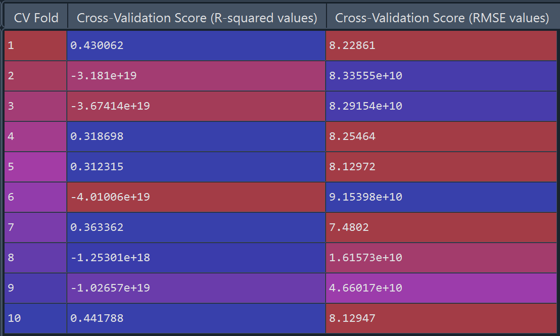
Below are the average results of R^2 and RMSE metrics after training using a linear regression model.

R-squared (R²) measures the proportion of the variance in the dependent variable (in this case, ‘popularity’) that is explained by the independent variables (features) in the model. As we know R^2 ranges from 0-1 with higher values indicating a better fit. This means the linear regression model is performing poorly.
The Root Mean Squared Error (RMSE) measures the average absolute error between the predicted values and the actual values. It provides a measure of how well the model’s predictions match the true values. Lower RMSE values indicate better model performance.
Based on these results the linear regression model is not a good fit. Let’s try a different model.
Step 5: Building a Ridge Regression Model
Import modules
from sklearn.linear_model import Ridge
Let’s select a range of alphas and instantiate the ridge model within the for loop
alphas = [0.1, 0.5, 0.75, 1.0, 1.25, 1.5, 2.0, 2.5]
for alpha in alphas:
    ridge = Ridge(alpha=alpha)
    # Perform cross-validation and obtain R-squared scores
       cv_scores = cross_val_score(ridge, X, y, cv=5, scoring='r2')

       # Calculate the average R-squared score across the 5 folds
       average_score = cv_scores.mean()

       # Calculate RMSE for each fold
       rmse_scores = np.sqrt(-cross_val_score(ridge, X, y, cv=5, scoring='neg_mean_squared_error'))
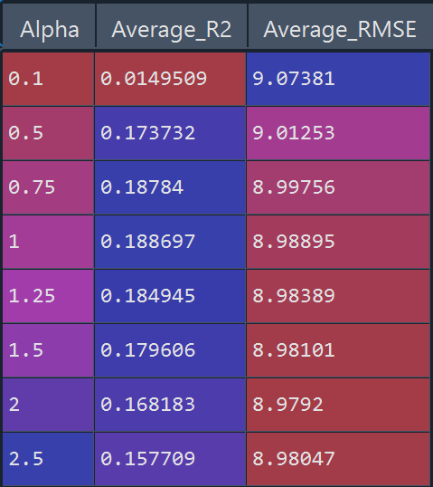
For each alpha the average (across the 5 cross folds) R^2 and RMSE value was saved in a table
Evaluating Ridge Regression Metrics
Using ridge regression the R^2 and RMSE metrics are as follows:
Average R^2 across alphas: 0.16
Average RMSE across alphas: 8.9
Recommendation
Ridge regression significantly reduced the RMSE, highlighting it’s ability to handle the limitations of linear regression.
The R^2 and RMSE values are of much more acceptable levels making ridge regression a more optimal model to predict the target variable, song popularity.
For more information head over to my Github